Socioeconomic Predictors of Anxiety: A Data Reuse Example Using NIH HEAL Datasets
This notebook demonstrates data reuse by combining data from two independent NIH HEAL studies that each collected anxiety scores using the GAD-2 (Generalized Anxiety Disorder 2-item) instrument alongside demographic variables.
About the Studies
The following datasets were used in this analysis. Please cite both the HEAL Data Platform record and the local repository when using these data.
- tDCS to Decrease Cravings in Patients with Opioid Use Disorder (HDP00619)
- This study examined transcranial Direct Current Stimulation (tDCS) as a treatment to reduce cravings in patients with Opioid Use Disorder (OUD) (Abrantes (2024)). The dataset used here contains baseline demographic and anxiety assessments collected at screening.
- Sensory Phenotyping to Enhance Neuropathic Pain Drug Development (HDP01233)
- This study characterized sensory phenotypes in patients with chronic neuropathic pain to inform drug development research (EDWARDS et al. (2026)). It includes demographic information and GAD-2 anxiety assessments collected across multiple study visits.
Why Combine Them?
Neither study alone provides enough participants for robust subgroup analysis. HDP00619 contributes 82 eligible records and HDP01233 contributes 199, giving a combined dataset of 281 participants drawn from two clinically distinct populations — OUD patients and chronic pain patients. Together, they offer greater statistical power to examine how age, sex, ethnicity, marital status, and employment relate to anxiety severity.
This combination is made possible by HEAL Common Data Elements (CDEs): standardized variable definitions shared across studies. Because both studies measured anxiety and demographics using the same standards, their data can be mapped to a common format and merged without manual column matching.
Full dataset citations are in the References section at the end of this notebook.
Research Questions
Is there a relationship between demographic variables and total anxiety scores?
Can we predict anxiety severity (GAD total score) using demographic features such as age, sex, ethnicity, marital status, and employment?
Can we classify individuals into high vs. low anxiety groups based on their demographic characteristics?
Which demographic and socioeconomic factors are most strongly associated with anxiety levels, and which are most important for predicting anxiety classification?
1. Imports and Setup
In this step, we import the tools needed for data analysis and modeling.
Pandas is used to handle tables of data (like Excel sheets).
NumPy helps with numerical calculations.
Matplotlib is used for creating visualizations such as graphs and charts.
train_test_split from scikit-learn helps divide the data into training and testing sets for building models.
We also have a library of helper functions in analysis_functions.py for:
Cleaning the datasets
Plotting graphs
Training machine learning models
Finally, we configure plotting settings to make the charts look clean and readable.
!pip install matplotlib scikit-learn -q
import pandas as pd
import numpy as np
import matplotlib.pyplot as plt
from sklearn.model_selection import train_test_split

from analysis_functions import *

# Configure matplotlib
plt.style.use('seaborn-v0_8-darkgrid')
plt.rcParams['figure.dpi'] = 100
1a. Download data for studies HDP00619 and HDP01233
import os, zipfile
# HDP00619
if not os.path.exists('208170/208170-V2/REDCap-Data/ProjectTHOUGHTUG3_FullREDCapDataset.csv'):
    !gen3 --endpoint=healdata.org drs-pull object dg.H35L/67fe6e34-bfc7-4c11-b6ed-b2f5702a401a
    with zipfile.ZipFile('ICPSR 208170/208170.zip', 'r') as archive:
        archive.extractall()
# HDP01233
if not os.path.exists('files/primary/SPENDD_UG3_demographicsFile.xlsx'):
    !gen3 drs-pull object dg.H34L/e380d743-cef7-4c92-8008-f4874246a478
if not os.path.exists('files/primary/SPENDD_UG3_Gad2.xlsx'):
    !gen3 drs-pull object dg.H34L/d7bb460c-93ab-4af3-9475-89d455e163cf
What Are Common Data Elements — and Why Do They Make Data Reuse Possible?
A Common Data Element (CDE) is a standardized definition for a variable: its name, data type, allowed values, and what those values mean. HEAL has defined CDEs for variables commonly used across pain and opioid use disorder research — including GAD-2 anxiety scores, age, sex, ethnicity, marital status, and employment status.
The file heal-mappings.json in the data folder that was downloaded from HEAL Semantic Search is the bridge that connects HEAL’s standard variable names to the specific column names used in each study. For example:
| HEAL Standard Variable | HDP00619 column | HDP01233 column |
|---|---|---|
Sex | gender | sex |
MARISTAT | marstat | maristat |
GAD2FeelNervScale | gad701 | gad2feelnervscale |
Without CDEs, you would need to manually read the data dictionary for each study, guess which columns correspond to the same measurement, reconcile different value encodings, and hope nothing was missed. That process doesn’t scale beyond 2–3 studies.
With CDEs, the mapping file does that work programmatically — making the combination process repeatable, auditable, and scalable to any number of studies that adopt the same standards.
The cleaning steps below use these mappings explicitly: the code looks up the study-specific column name from the standard ID, applies any necessary recoding, and then renames the column to the standard name — so both datasets end up with identical column names ready to merge.
2. Load, Standardize and Clean Data
Here we load data from two different studies:
HDP00619 — a CSV file with screening visit data
HDP01233 — two Excel files: one for demographics, one for GAD-2 responses
We first load the raw files and inspect them, then apply the CDE mappings to clean and standardize each dataset. After cleaning, both datasets will share identical column names and value encodings — a prerequisite for combining them.
print("Loading raw datasets...")
mappings     = load_mappings("../data/heal-mappings.json")
df_619_raw   = load_dataset("208170/208170-V2/REDCap-Data/ProjectTHOUGHTUG3_FullREDCapDataset.csv")
df_1233_demo = load_dataset("files/primary/SPENDD_UG3_demographicsFile.xlsx")
df_1233_gad  = load_dataset("files/primary/SPENDD_UG3_Gad2.xlsx")

print(f"\nHDP00619:              {df_619_raw.shape[0]:>4} rows, {df_619_raw.shape[1]:>3} columns")
print(f"HDP01233 demographics: {df_1233_demo.shape[0]:>4} rows, {df_1233_demo.shape[1]:>3} columns")
print(f"HDP01233 GAD-2:        {df_1233_gad.shape[0]:>4} rows, {df_1233_gad.shape[1]:>3} columns")

# Uncomment to preview raw data:
# display(df_619_raw.head(3))
# display(df_1233_demo.head(3))
# display(df_1233_gad.head(3))
Loading raw datasets...
HDP00619: 1488 rows, 692 columns
HDP01233 demographics: 203 rows, 19 columns
HDP01233 GAD-2: 404 rows, 5 columns
print("Cleaning HDP00619...")
df_619 = clean_hdp00619(df_619_raw.copy(), mappings)
print(f"  -> {len(df_619)} records after cleaning")
# display(df_619.head(3))

print("\nCleaning HDP01233...")
df_1233 = clean_hdp01233(df_1233_demo.copy(), df_1233_gad.copy(), mappings)
print(f"  -> {len(df_1233)} records after cleaning")
# display(df_1233.head(3))
Cleaning HDP00619...
Variable mappings for HDP00619:
Age -> 'age'
Sex -> 'gender'
ETHNIC -> 'ethnic'
MARISTAT -> 'marstat'
EMPSTAT -> 'empstat'
GAD2FeelNervScale -> 'gad701'
GAD2NotStopWryScale -> 'gad702'
-> 82 records after cleaning
Cleaning HDP01233...
Variable mappings for HDP01233:
Age -> 'age'
Sex -> 'sex'
ETHNIC -> 'ethnic'
MARISTAT -> 'maristat'
EMPSTAT -> 'empstat'
GAD2FeelNervScale -> 'gad2feelnervscale'
GAD2NotStopWryScale -> 'gad2notstopwryscale'
-> 199 records after cleaning
Notice that the two studies use different column names for the same variables (gender vs sex, gad701 vs gad2feelnervscale, marstat vs maristat), and HDP00619 has many columns not needed for this analysis. The cleaning step above used the CDE mappings to select, rename, and recode only the relevant columns — producing a standardized dataset from each study.
After cleaning, both datasets now use the HEAL standard variable names (Age, Sex, ETHNIC, MARISTAT, EMPSTAT, GAD2FeelNervScale, GAD2NotStopWryScale) and consistent integer encodings. This standardization is what makes combining them valid.
Comparing the datasets
We generate a scatter plot to visually compare the two datasets.
This helps us:
Check whether the datasets look similar
Identify differences in distributions
Detect any unusual patterns or outliers
Visualization is useful before combining datasets to ensure they are compatible.
# Scatter plot comparing both datasets
plot_scatter_comparison(df_619, df_1233, variable='Age', variable_label='Age (years)')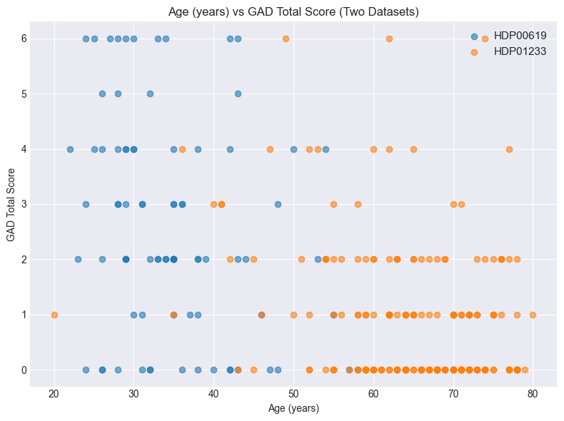
3. Merge the Datasets
After cleaning, both datasets share the same structure. We confirm record counts before combining, then concatenate into a single dataset for analysis.
A larger combined sample (N=281) gives us more statistical power than either study alone (HDP00619: N=82, HDP01233: N=199).
print(f"HDP00619 cleaned — {len(df_619)} records")
# display(df_619.head(3))

print(f"HDP01233 cleaned — {len(df_1233)} records")
# display(df_1233.head(3))

print("\nBoth datasets share the same columns and encodings — ready to combine.")
HDP00619 cleaned — 82 records
HDP01233 cleaned — 199 records
Both datasets share the same columns and encodings — ready to combine.
# Merge datasets
print("Merging datasets...")
df = pd.concat([df_619, df_1233], ignore_index=True)
print(f"Combined dataset shape: {df.shape}")
print(f"Total records: {len(df)}")
# df.head()
Merging datasets...
Combined dataset shape: (281, 9)
Total records: 281
4. Research Question 1: Is There a Relationship Between Demographic Variables and Anxiety?
This section addresses Research Question 1: Is there a relationship between demographic variables and total anxiety scores?
The panel below shows each demographic variable against the GAD total score. Age uses a scatter plot with a linear regression line; categorical variables use box plots showing the GAD score distribution per group.
# Label maps from HEAL standard variable definitions in heal-mappings.json
features = [
    ("Age",     "Age (years)",       None),
    ("Sex",     "Sex",               get_standard_labels("Sex",      mappings)),
    ("ETHNIC",  "Ethnicity",         get_standard_labels("ETHNIC",   mappings)),
    ("MARISTAT", "Marital Status",   get_standard_labels("MARISTAT", mappings)),
    ("EMPSTAT", "Employment Status", get_standard_labels("EMPSTAT",  mappings)),
]

fig, axes = plt.subplots(2, 3, figsize=(18, 10))
fig.suptitle("Demographic Features vs GAD Total Score", fontsize=14, fontweight="bold")

for ax, (feature, label, label_map) in zip(axes.flat, features):
    plot_feature_vs_gad(df, feature, label, ax=ax, label_map=label_map)

axes.flat[-1].set_visible(False)  # hide unused 6th subplot

plt.tight_layout()
plt.show()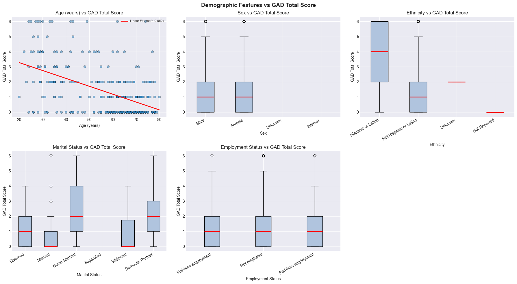
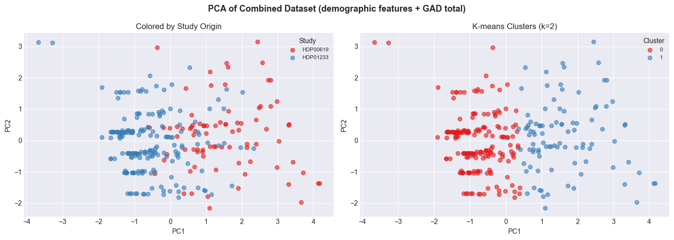
Cluster Analysis: Do Patterns Emerge Across the Two Populations?
Since the two studies recruited clinically distinct populations — OUD patients (HDP00619) and chronic pain patients (HDP01233) — it is worth asking whether these groups occupy separate regions of the feature space, or whether anxiety-driven patterns cut across study boundaries.
We use PCA to project the demographic + GAD features into 2D for visualization, and K-means (k=2) to find natural groupings. Two views of the same PCA projection are shown: colored by study origin, and colored by cluster assignment. If clusters largely align with study membership, the two populations are demographically distinct. If clusters cut across studies, it suggests shared anxiety-demographic profiles that transcend clinical context — a direct argument for the value of data reuse.
cluster_features = ['Age', 'Sex', 'ETHNIC', 'MARISTAT', 'EMPSTAT', 'gad_total']
study_labels = ['HDP00619'] * len(df_619) + ['HDP01233'] * len(df_1233)

cluster_labels, pca_coords, var_explained = run_kmeans(df, cluster_features, n_clusters=2)
print(f"PCA variance explained: PC1={var_explained[0]:.1%}, PC2={var_explained[1]:.1%}")

fig, axes = plt.subplots(1, 2, figsize=(14, 5))
fig.suptitle("PCA of Combined Dataset (demographic features + GAD total)", fontsize=13, fontweight='bold')
plot_pca_clusters(pca_coords, study_labels,           'Study',   'Colored by Study Origin',     ax=axes[0])
plot_pca_clusters(pca_coords, cluster_labels.tolist(), 'Cluster', 'K-means Clusters (k=2)',      ax=axes[1])
plt.tight_layout()
plt.show()
PCA variance explained: PC1=30.6%, PC2=17.0%
print("Cluster profiles — mean feature values per cluster:")
display(get_cluster_profiles(df, cluster_features, cluster_labels))

df_tmp = df.copy()
df_tmp['study']   = study_labels
df_tmp['cluster'] = cluster_labels
print("\nCluster composition by study (row proportions):")
display(pd.crosstab(df_tmp['cluster'], df_tmp['study'], normalize='index').round(2))
Cluster profiles — mean feature values per cluster:
Cluster composition by study (row proportions):
Interpreting this result: Check two things: (1) Does the left panel show clear separation by study? If yes, the populations are demographically distinct. (2) Do the clusters in the right panel align with study membership, or do they cut across it? Clusters that mix both studies around shared anxiety or demographic profiles are evidence that the combined dataset reveals patterns neither study could surface alone.
5. Prepare Data for Modeling
Machine learning models require numeric input features (X) and a target variable (y).
Here we create:
X → demographic variables (Age, Sex, Ethnicity, Marital Status, Employment Status)
y_linear → continuous anxiety score (
gad_total) for regressiony_logistic → binary high-anxiety indicator (
higher_anxiety) for classification
We also address class imbalance: only a small fraction of participants meet the high-anxiety threshold (GAD total ≥ 6). If ignored, models can achieve high accuracy by simply predicting “low anxiety” for everyone — which is useless in practice. We handle this in two ways:
Stratified train/test split — ensures the same proportion of high-anxiety cases appears in both the training and test sets, so the test set actually contains cases to evaluate
Balanced class weights — instructs the models to penalize errors on the minority class more heavily, so they are incentivized to learn to identify high-anxiety individuals
# Prepare features and targets
X, y_linear, y_logistic = prepare_model_data(df)

print("Features used in modeling:")
print(list(X.columns))
print(f"\nNumber of features: {X.shape[1]}")
print(f"Number of samples: {X.shape[0]}")
# X.head()
Features used in modeling:
['Age', 'Sex', 'MARISTAT', 'EMPSTAT', 'ETHNIC']
Number of features: 5
Number of samples: 281
# Split data into training and test sets
# stratify=y_logistic ensures both sets have the same proportion of high-anxiety cases
X_train, X_test, y_train_lin, y_test_lin = train_test_split(
    X, y_linear, test_size=0.2, random_state=42, stratify=y_logistic
)

_, _, y_train_log, y_test_log = train_test_split(
    X, y_logistic, test_size=0.2, random_state=42, stratify=y_logistic
)

X_train = X_train.fillna(0)
X_test  = X_test.fillna(0)

print(f"Training set size: {len(X_train)}")
print(f"Test set size:     {len(X_test)}")
print(f"\nHigh-anxiety rate — train: {y_train_log.mean():.1%}  |  test: {y_test_log.mean():.1%}")
print("(These should be similar, confirming the stratified split worked.)")
Training set size: 224
Test set size: 57
High-anxiety rate — train: 4.5% | test: 5.3%
(These should be similar, confirming the stratified split worked.)
6. Research Question 2: Linear Regression for Predicting Anxiety using Demographic Features
This section addresses Research Question 2: Can we predict anxiety severity (GAD total score) using demographic features such as age, sex, ethnicity, marital status, and employment?
Training linear regression model
Linear regression predicts continuous anxiety scores.
The model learns how demographic variables influence anxiety level using the GAD total score.
We evaluate using:
R² Score → how well the model explains variation
RMSE → average prediction error
This helps understand predictive power.
# Train linear regression model
lin_results = train_linear_regression(X_train, y_train_lin, X_test, y_test_lin)

print("Linear Regression Results")
print("=" * 50)
print(f"R² Score: {lin_results['r2']:.4f}")
print(f"RMSE: {lin_results['rmse']:.4f}")
Linear Regression Results
==================================================
R² Score: 0.3186
RMSE: 1.3593
Interpreting this result: The R² score measures how much of the variation in anxiety scores the model explains — 0 means no explanatory power, 1 means perfect. The result here shows demographics account for a meaningful but partial share of anxiety variation. Clinical history, treatment context, and psychological factors likely explain much of what remains. The RMSE gives the average prediction error in the original 0–6 GAD score units — a useful sanity check on whether the model’s predictions are in a plausible range.
Visualize Linear Regression Coefficients
The coefficient plot shows the direction and strength of each feature’s linear association with the GAD total score:
Positive coefficient → higher values of that feature are associated with higher anxiety
Negative coefficient → higher values are associated with lower anxiety
Larger magnitude → stronger linear association
This is part of interpreting the regression model. Section 9 will revisit feature importance from a different angle — using random forest — so you can compare the two perspectives side by side.
# Plot linear regression coefficients
coefficients = plot_linear_coefficients(lin_results['model'], X)
print("\nLinear Regression Coefficients:")
print(coefficients)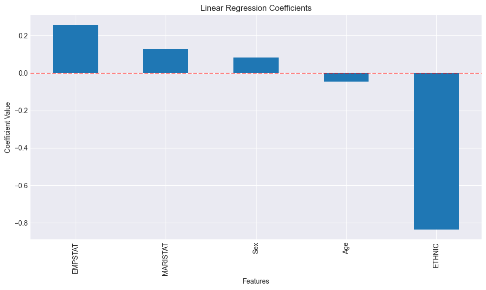
Linear Regression Coefficients:
EMPSTAT     0.255900
MARISTAT    0.128800
Sex         0.082902
Age        -0.046500
ETHNIC     -0.835257
dtype: float64
Interpreting this result: Features with larger absolute coefficients have a stronger linear association with anxiety scores. A positive coefficient means higher values of that variable predict higher anxiety; negative means lower. Note that these are associations, not causes — a coefficient for ethnicity, for example, likely reflects structural and social factors rather than ethnicity itself.
7. Research Question 3: Classifying Individuals into High vs. Low Anxiety
This section addresses Research Question 3: Can we classify individuals into high vs. low anxiety groups based on their demographic characteristics?
Training Logistic Regression Model
Logistic regression predicts categories, such as:
High anxiety
Low anxiety
Evaluation metrics:
Accuracy
Confusion matrix
Classification report (precision, recall, F1)
This model helps classify participants into risk groups.
# Train logistic regression model
log_results = train_logistic_regression(X_train, y_train_log, X_test, y_test_log)

print("Logistic Regression Results")
print("=" * 50)
print(f"Accuracy: {log_results['accuracy']:.4f}")
print("\nConfusion Matrix:")
print(log_results['confusion_matrix'])
print("\nClassification Report:")
print(log_results['classification_report'])
Logistic Regression Results
==================================================
Accuracy: 0.7544
Confusion Matrix:
[[41 13]
[ 1 2]]
Classification Report:
precision recall f1-score support
0 0.98 0.76 0.85 54
1 0.13 0.67 0.22 3
accuracy 0.75 57
macro avg 0.55 0.71 0.54 57
weighted avg 0.93 0.75 0.82 57
Interpreting this result: Look beyond the headline accuracy. With balanced class weights, the confusion matrix should now show the model identifying some high-anxiety individuals rather than predicting everyone as low-anxiety. Precision, recall, and F1 for the high-anxiety class (class 1) are the meaningful metrics here — accuracy alone is misleading when classes are imbalanced.
8. Decision Tree Classifier (Research Question 3, cont.)
A decision tree is a second approach to Research Question 3. Unlike logistic regression, which finds a linear decision boundary, a decision tree splits the data recursively based on thresholds in individual features — producing explicit if/then rules that are easy to interpret.
Advantages:
Each split is a plain decision rule, readable by non-technical audiences
Handles nonlinear relationships naturally
No assumption that features combine linearly
We compare its performance to logistic regression to see whether a nonlinear approach improves detection of high-anxiety cases.
# Train decision tree
tree_results = train_decision_tree(X_train, y_train_log, X_test, y_test_log, X)

print("Decision Tree Results")
print("=" * 50)
print(f"Accuracy: {tree_results['accuracy']:.4f}")
Decision Tree Results
==================================================
Accuracy: 0.9474
Visualizing Decision Tree Structure
This visualization shows:
How decisions are made
Which features are used first
Decision thresholds
This is helpful for explaining results to non-technical audiences.
# Visualize decision tree
plot_decision_tree(tree_results['model'], tree_results['feature_names'])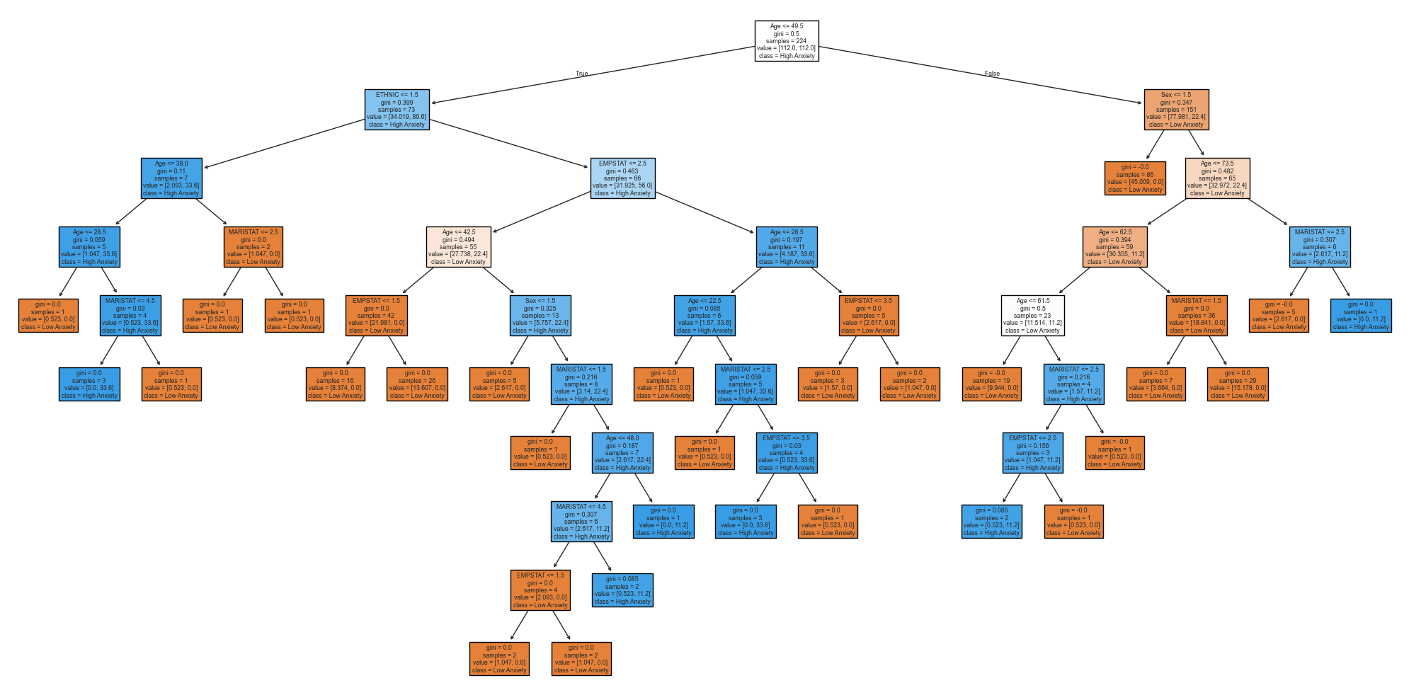
Interpreting this result: The decision tree accuracy can be compared to logistic regression to see whether a non-linear decision boundary improves classification. The tree visualization above shows the exact rules the model learned — a useful feature when explaining findings to clinicians or non-technical stakeholders.
9. Research Question 4: Which Factors Are Most Associated with and Predictive of Anxiety?
This section addresses Research Question 4: Which demographic and socioeconomic factors are most strongly associated with anxiety levels, and which are most important for predicting anxiety classification?
The linear regression coefficients in Section 6 gave one answer: which variables have the strongest linear association with the continuous GAD score. Here we get a complementary answer using random forest feature importance, which measures how useful each variable is for correctly splitting the data into high vs. low anxiety groups across an ensemble of decision trees. Comparing the two gives a fuller picture — a variable can have a large regression coefficient but low forest importance (or vice versa), and understanding that difference is informative.
# Train random forest
rf_results = train_random_forest(X_train, y_train_log, X_test, y_test_log)

print("Random Forest Results")
print("=" * 50)
print(f"Accuracy: {rf_results['accuracy']:.4f}")
Random Forest Results
==================================================
Accuracy: 0.9474
Interpreting this result: Random forest aggregates many decision trees to reduce overfitting. Compare its confusion matrix to the logistic regression — if it better captures high-anxiety cases, the ensemble approach is providing value. Accuracy alone is not the right metric here given the class imbalance.
Identifying Most Important Features
Random forest calculates feature importance.
This shows:
Which variables influence predictions most
Key drivers of anxiety
Variables worth further investigation
This step helps summarize findings.
# Plot feature importance
importance = plot_feature_importance(rf_results['model'], X)
print("\nFeature Importance:")
print(importance)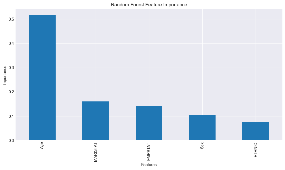
Feature Importance:
Age         0.516668
MARISTAT    0.161165
EMPSTAT     0.142664
Sex         0.103925
ETHNIC      0.075578
dtype: float64
Interpreting this result: Feature importance scores sum to 1. A dominant score for Age means the model found age to be the most useful splitter across all trees. However, high importance does not imply causation, and importance can be inflated for continuous variables (like age) relative to binary ones. The relative ranking across features is more meaningful than the absolute scores.
10. Answers to Research Questions
Based on our analysis, here are the answers to our research questions:
print("=" * 80)
print("ANSWERS TO RESEARCH QUESTIONS")
print("=" * 80)
print()

print("Q1: Is there a relationship between demographic variables and total anxiety scores?")
print()
print("ANSWER: Yes. The feature panel (Section 4) shows:")
print("  - Age has a slight negative linear relationship with GAD total score")
print("  - Categorical features (Sex, Ethnicity, Marital Status, Employment)")
print("    show varying GAD distributions across groups — see box plots for details")
print()

print("Q2: Can we predict anxiety severity (GAD total score) using demographic features?")
print()
print(f"ANSWER: Yes, with moderate success. The Linear Regression model achieved:")
print(f"  - R\u00b2 Score: {lin_results['r2']:.4f}")
print(f"  - RMSE: {lin_results['rmse']:.4f}")
print(f"  Demographic features explain approximately {lin_results['r2']*100:.1f}% of the")
print(f"  variance in anxiety scores — a modest but meaningful signal.")
print()

print("Q3: Can we classify individuals into high vs. low anxiety groups?")
print()
print(f"ANSWER: Classification performance:")
print(f"  - Logistic Regression Accuracy: {log_results['accuracy']:.4f}")
print(f"  - Decision Tree Accuracy:       {tree_results['accuracy']:.4f}")
print(f"  - Random Forest Accuracy:       {rf_results['accuracy']:.4f}")
print(f"  Note: headline accuracy is high but misleading due to class imbalance.")
print(f"  The F1 score for the high-anxiety class is the more meaningful metric.")
print()

print("Q4: Which factors are most strongly associated with anxiety, and most")
print("    important for predicting anxiety classification?")
print()
print("  Linear regression — strongest associations (by absolute coefficient):")
top_coef_idx = coefficients.abs().sort_values(ascending=False).head(3).index
for i, feature in enumerate(top_coef_idx, 1):
    coef = coefficients[feature]
    direction = "positive" if coef > 0 else "negative"
    print(f"    {i}. {feature}: {direction} (coefficient: {coef:.4f})")
print()
print("  Random Forest — top predictive features (by importance):")
top_3_features = importance.head(3)
for i, (feature, imp) in enumerate(top_3_features.items(), 1):
    print(f"    {i}. {feature} (importance: {imp:.4f})")
print()
================================================================================
ANSWERS TO RESEARCH QUESTIONS
================================================================================
Q1: Is there a relationship between demographic variables and total anxiety scores?
ANSWER: Yes. The feature panel (Section 4) shows:
- Age has a slight negative linear relationship with GAD total score
- Categorical features (Sex, Ethnicity, Marital Status, Employment)
show varying GAD distributions across groups — see box plots for details
Q2: Can we predict anxiety severity (GAD total score) using demographic features?
ANSWER: Yes, with moderate success. The Linear Regression model achieved:
- R² Score: 0.3186
- RMSE: 1.3593
Demographic features explain approximately 31.9% of the
variance in anxiety scores — a modest but meaningful signal.
Q3: Can we classify individuals into high vs. low anxiety groups?
ANSWER: Classification performance:
- Logistic Regression Accuracy: 0.7544
- Decision Tree Accuracy: 0.9474
- Random Forest Accuracy: 0.9474
Note: headline accuracy is high but misleading due to class imbalance.
The F1 score for the high-anxiety class is the more meaningful metric.
Q4: Which factors are most strongly associated with anxiety, and most
important for predicting anxiety classification?
Linear regression — strongest associations (by absolute coefficient):
1. ETHNIC: negative (coefficient: -0.8353)
2. EMPSTAT: positive (coefficient: 0.2559)
3. MARISTAT: positive (coefficient: 0.1288)
Random Forest — top predictive features (by importance):
1. Age (importance: 0.5167)
2. MARISTAT (importance: 0.1612)
3. EMPSTAT (importance: 0.1427)
- Abrantes, A. (2024). tDCS to Decrease Cravings in patients with OUD in the United States [February 2023]. ICPSR - Interuniversity Consortium for Political. 10.3886/E208170V2
- EDWARDS, R. R., FREEMAN, R., & Gewandter, J. (2026). Sensory Phenotyping to Enhance Neuropathic Pain Drug Development. HEAL Data Platform. 10.60490/HDP01233